A credit risk is the risk of default on a debt that may arise from a borrower failing to make required payments. In the first resort, the risk is that of the lender and includes lost principal and interest, disruption to cash flows, and increased collection costs. We’ll focuse on retail banking area.
The dataset from Banque de France is composed of 10 features and 99.302 customers.
We’ll procede first to load packages and functions, and work on light data processing. At the end we’ll implement deep learning model and check output model indicators.
Configuation packages / functions
Packages: we load 5 packages for data processing, train deep learning model and indicators output
# packages
library(data.table) # for data processing
library(dummies) # for data processing
library(tensorflow) # for classification
library(keras) # for classification
library(ROCR) # to measure model performance
Functions: functions for data processing & output model indicators
# compute lift
whatsMyLift <- function(score,cible, perc = 0.1,target){

  n = ceiling(perc*length(score))
  percentile = cible[order(score, decreasing = T)[1:n]]
  length(percentile[percentile==target])/length(cible[cible==target])
}

# compute gini + lift
IndicatorsModels<-function(base,proba,target){

  pred <- prediction(proba, FactorToBinNum(base$target,target))
  perf <- performance(pred, measure = "tpr", x.measure = "fpr")
  auc <- performance(pred, measure = "auc")
  GiniIndex<-as.numeric(auc@y.values[[1]]*2-1)
  plot(perf)
  L5<-whatsMyLift(proba,base$target,perc=0.05,target)
  L10<-whatsMyLift(proba,base$target,perc=0.1,target)
  ResInd<-c(L5,L10,GiniIndex)
  names(ResInd)<-c("Lift5","Lift10","gini")
  round(ResInd*100,0)
}

# normalize vector
normalize <- function(x) {

  ((x - min(x)) / (max(x) - min(x)))
}

# transform vector
BinToFactor<-function(vect,NonTarget,target){

  vect[vect==0]<-NonTarget
  vect[vect==1]<-target
  as.factor(vect)
}

# transform vector
FactorToBin<-function(vect,target){
  vect<-as.character(vect)
  vect[vect!=target]<-"0"
  vect[vect==target]<-"1"
  as.factor(vect)
}

# transform vector
FactorToBinNum<-function(vect,target){
  vect<-as.character(vect)
  vect[vect!=target]<-"0"
  vect[vect==target]<-"1"
  as.numeric(vect)
}

# split train/test
trainTestSplit <- function(df,trainPercent,seed1){
  ## sample size percent
  samp_size <- floor(trainPercent/100 * nrow(df))
  ## set the seed
  set.seed(seed1)
  idx <- sample(seq_len(nrow(df)), size = samp_size)
  idx
}

PropTable2<-function(vect){
  round(prop.table(table(vect)),2)
}
Data processing
Reading credit risk dataset. We use fread function from data.table package (fast read).
path<-paste(getwd(),"data",sep="/")
data<-fread(paste(path,"dataset.csv",sep="/"),sep=";",stringsAsFactors = F,colClasses = "character")
data<-data.frame(data)
Processing numerical & factor features. We’ll scale et replace NA value for numerical features, and dummies the categorical features.
# select data
ListNum<-c("amount","old.work","default","time","downpayment")
ListFact<-c("type","type.work","gender","working.sector","used.car")

# numerical features processing: NA & scale
DataNum<-data[,match(ListNum,names(data))]
for (i in 1:dim(DataNum)[2]){
  col<-as.numeric(DataNum[,i])
  col[is.na(col)]<-median(col[!is.na(col)])
  col<-normalize(col)
  DataNum[,i]<-col
}
str(DataNum)
'data.frame':   99392 obs. of  5 variables:
 $ amount     : num  0.506 0.509 0.449 0.503 0.405 ...
 $ old.work   : num  0.327 0.232 0.048 0.166 0.156 ...
 $ default    : num  0 0 0 0 0 0 0 0 0 0 ...
 $ time       : num  0.514 0.667 0.667 0.5 0.167 ...
 $ downpayment: num  0 0 0.434 0 0.716 ...
# factor features processing
DataFact<-data[,match(ListFact,names(data))]
for (i in 1:dim(DataFact)[2]){
  col<-as.factor(DataFact[,i])
  DataFact[,i]<-col
}
str(DataFact)
'data.frame':   99392 obs. of  5 variables:
 $ type          : Factor w/ 2 levels "PRI","PRO": 2 2 1 2 1 1 1 2 2 1 ...
 $ type.work     : Factor w/ 17 levels "","0","10","11",..: 6 2 6 6 4 5 4 2 4 6 ...
 $ gender        : Factor w/ 7 levels "","C","D","M",..: 4 2 2 4 4 4 4 2 2 2 ...
 $ working.sector: Factor w/ 17 levels "AGR","ATR","BTP",..: 10 1 2 10 3 4 2 1 3 2 ...
 $ used.car      : Factor w/ 2 levels "VN","VO": 1 1 1 1 1 1 1 1 1 1 ...
# decompose factor dataset on dummy
DataFact<-dummy.data.frame(DataFact,sep="-")
Final dataset: merge between numerical and dummies features.
# final data
data<-data.frame(DataNum,DataFact)

# numerical format
for (i in 1:dim(data)[2]){
  data[,i]<-as.numeric(data[,i])
}
Define the target: we just rename the target.
# define target
names(data)[match("default",names(data))]<-"target"

# target proportion
PropTable2(data$target)
vect
   0    1
0.98 0.02
We see umbalanced data, we have two ways here: first we work with umbalanced data on the algorithm or we work now on the data to get balanced.
Umbalanced data
We have to deal with the umbalanced dataset: we’ll generate artifical data to get balanced.
# take umbalanced data
DataTarget<-data[data$target==1,]
d1<-dim(DataTarget)[1]
d2<-dim(data)[1]
t<-round(d2/d1,0)
res<-NULL
for (i in 1:t){
  res<-rbind(res,DataTarget)
}
data<-rbind(data,res)

# mixed data
Random<-557
data_idx<-trainTestSplit(data,100,Random)
data<-data[data_idx,]

# proportion with balanced data
PropTable2(data$target)
vect
   0    1
0.49 0.51
Split dataset
We just rename the target as “Default” or “NonDefault”
# named target
NonTarget<-"NonDefault"
target<-"default"

# change target to names
data$target<-BinToFactor(data$target,NonTarget,target)
Split train/test set: we take 70% of train and 30% of test set
# named target
NonTarget<-"NonDefault"
target<-"default"

# change target to names
data$target<-BinToFactor(data$target,NonTarget,target)

# train and test
Random<-558
train_idx <- trainTestSplit(data,70,Random)
train <- data[train_idx, ]
test <- data[-train_idx, ]

# check target proportion on train/test dataset
r1<-PropTable2(train$target)
r2<-PropTable2(test$target)
r3<-rbind(r1,r2)
rownames(r3)<-c("train","test")
print(r3)
      default NonDefault
train    0.51       0.49
test     0.51       0.49
Processing final data for tensorflow format model
# match target
mTarget<-match("target",names(data))

# data processing for tensorflow
x_train <- data.matrix(train[,-mTarget])
x_test <- data.matrix(test[,-mTarget])
y_train <- as.numeric(FactorToBin(train$target,target))-1
y_train <- to_categorical(y_train, 2)
y_test <- as.numeric(FactorToBin(test$target,target))-1
y_test <- to_categorical(y_test, 2)
Model
Set up sequential neural network model using Keras API. The sequential model makes the assumption that the network has exactly one input and exactly one output, and that it consists of a linear stack of layers.
- layer_dense: This layer can be interpreted as a function, which takes as input a 2D tensor and returns another 2D tensor—a new representation for the input tensor. Specifically, the function is as follows (where W is a 2D tensor and b is a vector, both attributes of the layer) output = relu(dot(W, input) + b) with dot product: between the input tensor and a tensor named W, vector b and relu: relu(x) is max(x, 0)
- activation function: Without an activation function like relu (also called a non-linearity), the dense layer would consist of two linear operations—a dot product and an addition: output = dot(W, input) + b So the layer could only learn linear transformations (affine transformations) of the input data: the hypothesis space of the layer would be the set of all possible linear transformations of the input data into a 16-dimensional space. Such a hypothesis space is too restricted and wouldn’t benefit from multiple layers of representations, because a deep stack of linear layers would still implement a linear operation: adding more layers wouldn’t extend the hypothesis space. In order to get access to a much richer hypothesis space that would benefit from deep representations, you need a non-linearity, or activation function. relu is the most popular activation function in deep learning, but there are many other candidates, which all come with similarly strange names: prelu, elu, and so on.
- input_shape: dimensionality of the input (integer) not including the samples axis. This argument is required when using this layer as the first layer in a model.
- layer_dropout: consists in randomly setting a fraction rate of input units to 0 at each update during training time, which helps prevent overfitting.
# dimension dataset
d<-dim(train)[2]-1

# set up model
model <- keras_model_sequential()
model %>%
  layer_dense(units = 5, activation = 'relu', input_shape = d) %>%
  layer_dropout(rate = 0.1) %>%
  layer_dense(units = 7, activation = 'relu', input_shape = d) %>%
  layer_dropout(rate = 0.1) %>%
  layer_dense(units = 7, activation = 'relu', input_shape = d) %>%
  layer_dropout(rate = 0.1) %>%
layer_dense(units = 2, activation = 'softmax')- Compile: to make the network ready for training, we need to pick three more things, as part of the compilation step:
- Loss function: how the network will be able to measure its performance on the training data, and thus how it will be able to steer itself in the right direction.
- Optimizer: the mechanism through which the network will update itself based on the data it sees and its loss function.
- Metrics: to monitor during training and testing.
# compile model
model %>% compile(
  loss = 'categorical_crossentropy',
  optimizer = optimizer_rmsprop(),
  metrics = 'accuracy'
)
print(model)
Model
______________________________________________________________________
Layer (type)                   Output Shape                Param #
======================================================================
dense_1 (Dense)                (None, 5)                   250
______________________________________________________________________
dropout_1 (Dropout)            (None, 5)                   0
______________________________________________________________________
dense_2 (Dense)                (None, 7)                   42
______________________________________________________________________
dropout_2 (Dropout)            (None, 7)                   0
______________________________________________________________________
dense_3 (Dense)                (None, 7)                   56
______________________________________________________________________
dropout_3 (Dropout)            (None, 7)                   0
______________________________________________________________________
dense_4 (Dense)                (None, 2)                   16
======================================================================
Total params: 364
Trainable params: 364
Non-trainable params: 0
______________________________________________________________________- Train your model
- epoch: number of iteration over all samples in the x_train and y_train tensors
- batch_size: mini batches
- validation_split: set of validation
# fit model
history <- model %>% fit(
  x_train, y_train,
  epochs = 20, batch_size = 100,
  validation_split = 0.2
)
print(history)
Trained on 110,964 samples, validated on 27,742 samples (batch_size=100, epochs=20)
Final epoch (plot to see history):
val_loss: 0.5481
 val_acc: 0.7107
    loss: 0.559
     acc: 0.7135
Result of training
plot(history)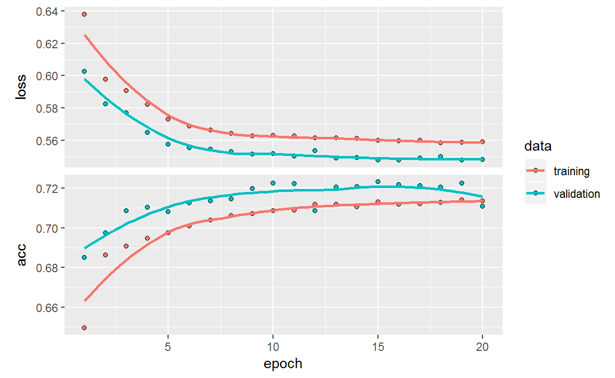
Model indicators
AUC is common metric on credit risk: AUC is area under the curve, In a ROC curve the true positive rate (Sensitivity) is plotted in function of the false positive rate (100-Specificity) for different cut-off points of a parameter. We’ll compute gini index: gini = 2*AUC-1.
model %>% evaluate(x_test, y_test)
$loss
[1] 0.5422537

$acc
[1] 0.7153551
proba<-model %>% predict_proba(x_train)
proba<-proba[,2]
hist(proba)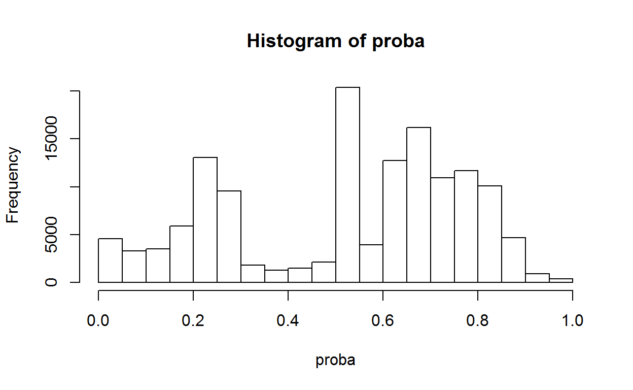
ResTrain<-IndicatorsModels(train,proba,target)["gini"]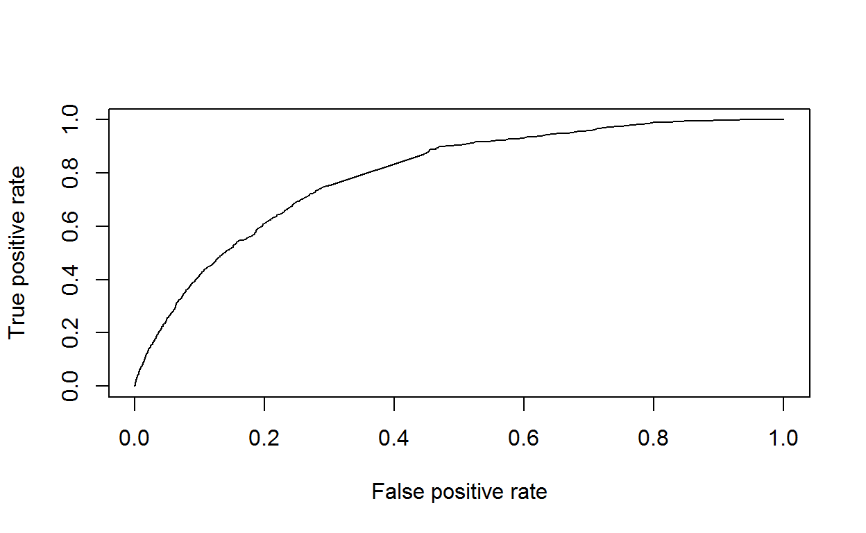
proba<-model %>% predict_proba(x_test)
proba<-proba[,2]
hist(proba)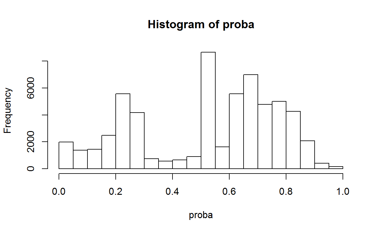
ResTest<-IndicatorsModels(test,proba,target)["gini"]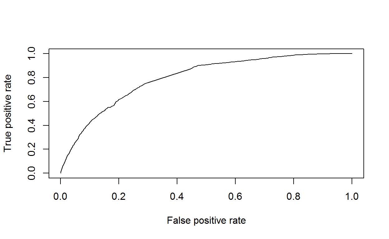
res<-rbind(ResTrain,ResTest)
rownames(res)<-c("train","test")
print(res)
      gini
train   59
test    59
The gini index for train set is very close to test set, it’s a good thing. But the value of the index is bigger than 50%, it’s good result. Our model have a good predictive ability.
This example show how to use Keras API for binary classification and to measure the model performance with AUC.